Gradient Descent

Image extracted from: Creating a Gradient Descent Animation in Python

Gradient descent is one of the most fundamental optimization algorithms in machine learning. It's a method for finding the minimum of a function by iteratively moving in the direction of steepest descent.

The Intuition

Imagine you're standing on a mountain in thick fog, and you want to reach the valley below. You can't see far, but you can feel the slope beneath your feet. Gradient descent works the same way: it takes small steps downhill, following the steepest path, until it reaches a minimum.

The Mathematics

The Basic Formula

At its core, gradient descent updates parameters using this simple formula:

Where:

• $\theta$ represents the parameters we're optimizing
• $\alpha$ is the learning rate (step size)
• $\nabla J(\theta)$ is the gradient of the cost function $J$ with respect to $\theta$

Understanding the Gradient: From Simple to Complex

Let's demystify the gradient symbol $\nabla$ (called "nabla" or "del") by building up from the simplest case.

Case 1: Single Variable (One Parameter)

When we have just one parameter, the gradient is simply the derivative:

The derivative tells us: "If I increase $\theta$ by a tiny amount, how much does $J$ change?"

Example: For $J(\theta) = \theta^2$:

• If $\theta = 5$, then $\nabla J(5) = 10$ → function is increasing, go left (decrease $\theta$)
• If $\theta = -3$, then $\nabla J(-3) = -6$ → function is decreasing, go right (increase $\theta$)
• If $\theta = 0$, then $\nabla J(0) = 0$ → we're at the minimum!

Case 2: Two Variables (Two Parameters)

When we have two parameters $\theta_1$ and $\theta_2$, the gradient becomes a vector with two components:

Each partial derivative $\frac{\partial J}{\partial \theta_i}$ asks: "If I change only $\theta_i$ (keeping others fixed), how much does $J$ change?"

Example: For $J(\theta_1, \theta_2) = \theta_1^2 + \theta_2^2$:

At point $(\theta_1=3, \theta_2=4)$:

This vector points in the direction of steepest ascent. We go in the opposite direction (subtract it) to descend!

Case 3: Many Variables (General Case)

For n parameters $\theta_1, \theta_2, \ldots, \theta_n$, the gradient is an n-dimensional vector:

Each component tells us how sensitive $J$ is to changes in that specific parameter. This is exactly what we need to know which direction to adjust each parameter!

Key Insight: Whether you have 1 parameter or 1 million parameters, the idea is the same: compute how much each parameter affects the cost, then adjust them in the opposite direction.

Walking Through a Complete Example

Let's see gradient descent in action with the simplest case: one variable.

Consider minimizing the quadratic function:

The gradient (derivative) is:

The gradient descent update rule becomes:

Starting at $\theta_0 = 10$ with learning rate $\alpha = 0.1$:

Iteration 1:

The gradient was positive (10 slope upward), so we moved left (decreased $\theta$)

Iteration 2:

Still positive gradient, getting smaller, so smaller steps

Iteration 3:

Pattern continues: as we approach the minimum, the gradient shrinks, so our steps get smaller automatically!

With each step, we get closer to the minimum at $\theta = 0$. Notice how the steps naturally get smaller as the gradient decreases near the minimum.

Key Concepts

Learning Rate

The learning rate $\alpha$ is crucial:

• Too large: We might overshoot the minimum or even diverge
• Too small: Convergence will be very slow
• Just right: Efficient convergence to the minimum

Let's do experiments with different learning rates and see how it affects convergence!

Types of Gradient Descent

1. Batch Gradient Descent

Uses the entire dataset to compute the gradient:

Where $J(\theta)$ is computed over all training examples.

2. Stochastic Gradient Descent (SGD)

Updates parameters using one training example at a time:

3. Mini-batch Gradient Descent

A compromise: uses a small batch of examples:

Where $b$ is the batch size.

Convergence

Gradient descent converges when the gradient becomes very small:

Where $\epsilon$ is a small threshold value.

Challenges

1. Local Minima: The algorithm might get stuck in local minima instead of finding the global minimum
2. Saddle Points: Points where the gradient is zero but aren't minima
3. Plateau Regions: Areas where the gradient is very small, slowing down learning

Real-World Applications

Gradient descent is used to train:

• Neural Networks: Optimizing millions of parameters
• Linear Regression: Finding the best-fit line
• Logistic Regression: Classification problems
• Support Vector Machines: Finding optimal hyperplanes

Gradient Descent in Deep Learning

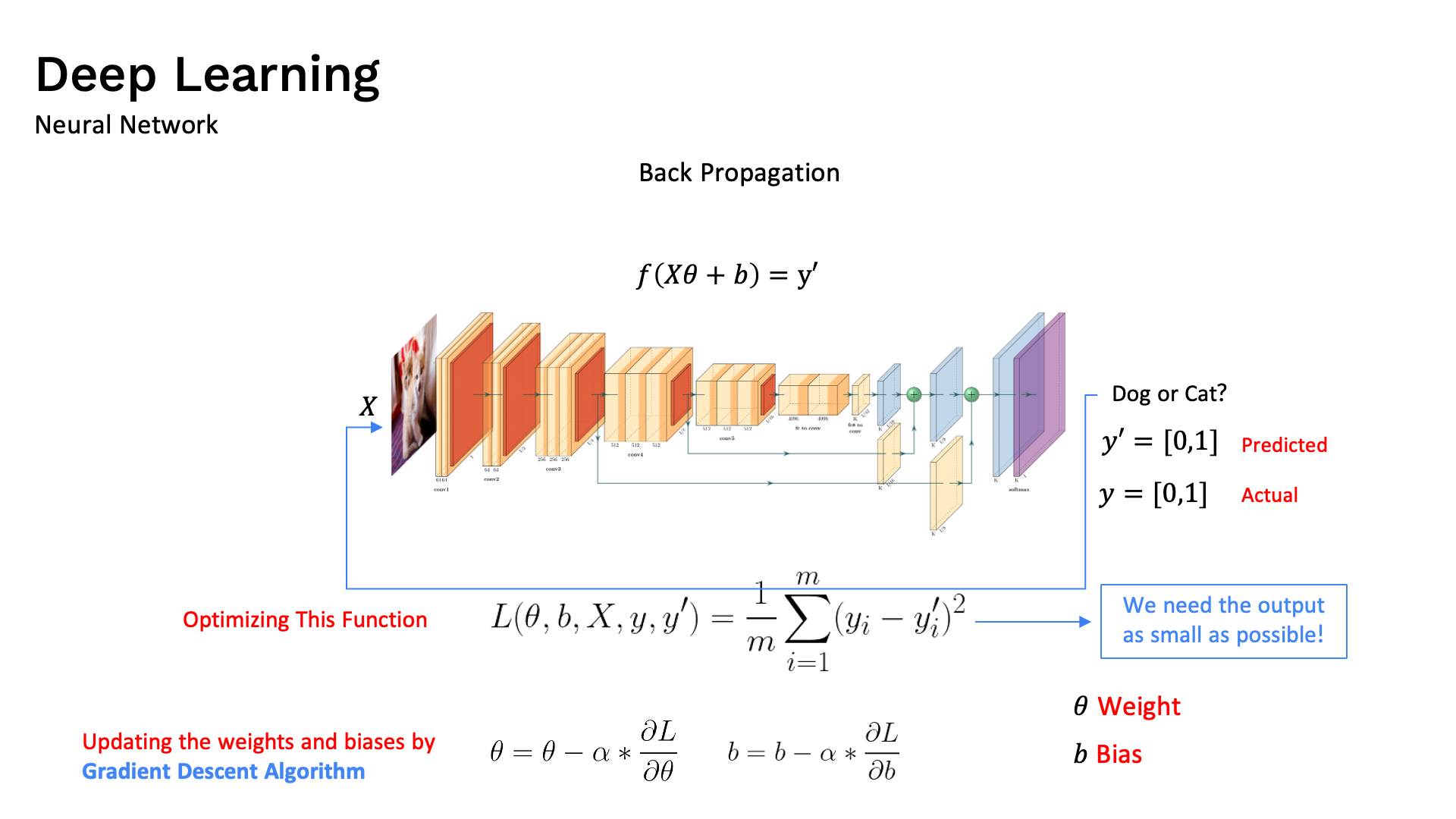
A deep neural network uses gradient descent to train weights across all its layers by minimizing the cost function.

The image above shows a Deep Neural Network — a powerful type of model that directly relies on gradient descent to optimize its cost function.

In deep learning:

• Input Layer receives raw data (e.g. image pixels, words, numbers)
• Hidden Layers perform feature extraction — learning complex patterns from data
• Output Layer produces the final prediction
• Weights $w$ in each connection are the parameters $\theta$ that gradient descent optimizes

During training, the process is:

A network may have millions of neurons → millions of weights → a gradient vector with millions of dimensions — yet gradient descent works exactly the same way as in the 1D case: move opposite to the gradient to reduce the loss!

Python Implementation

Below is a pure-Python implementation — no ML libraries. Each block maps directly to the math above. Highlighted lines are the core formulas.

Step 1 — Cost Function and its Gradient

$J(\theta) = \theta^2, \qquad \nabla J(\theta) = 2\theta$

# J(θ) = θ²  →  the function we want to minimize
def cost(theta):
    return theta ** 2

# ∇J(θ) = dJ/dθ = 2θ  →  its derivative (gradient)
def gradient(theta):
    return 2 * theta

Step 2 — The Update Rule

$\theta_{new} = \theta_{old} - \alpha \cdot \nabla J(\theta)$

def update(theta, alpha):
    grad = gradient(theta)           # ① compute  ∇J(θ)
    return theta - alpha * grad      # ② apply   θ_new = θ_old − α·∇J(θ)

Line 3 is the update rule formula above, written directly as Python.

Step 3 — Full Loop Until Convergence

Run updates until $|\nabla J(\theta)| < \varepsilon$ — when the gradient is essentially zero:

def gradient_descent(theta_init, alpha, epsilon=1e-6, max_iters=1000):
    theta = theta_init                           # θ₀ — starting point
    for i in range(max_iters):
        grad = gradient(theta)                   # ∇J(θ) = 2θ
        if abs(grad) < epsilon:                  # stop when |∇J(θ)| < ε
            print(f"Converged at iteration {i}")
            break
        theta = theta - alpha * grad             # θ_new = θ_old − α·∇J(θ)
        if i < 5:
            print(f"  iter {i+1:2d}: θ={theta:.5f}  J={cost(theta):.5f}  ∇J={grad:.5f}")
    return theta

# Same starting values as the manual example above: θ₀ = 10, α = 0.1
theta_min = gradient_descent(theta_init=10.0, alpha=0.1)
print(f"\nMinimum at θ = {theta_min:.8f}")

Output — matches the manual iterations above:

  iter  1: θ= 8.00000  J=64.00000  ∇J=20.00000
  iter  2: θ= 6.40000  J=40.96000  ∇J=16.00000
  iter  3: θ= 5.12000  J=26.21440  ∇J=12.80000
  iter  4: θ= 4.09600  J=16.77722  ∇J=10.24000
  iter  5: θ= 3.27680  J=10.73742  ∇J= 8.19200
Minimum at θ = 0.00000001

Step 4 — Linear Regression: Two Parameters

For a model $\hat{y} = wX + b$, the cost is mean squared error:

$J(w, b) = \frac{1}{m} \sum_{i=1}^{m} \left(\hat{y}^{(i)} - y^{(i)}\right)^2$

With partial derivatives:

$\frac{\partial J}{\partial w} = \frac{2}{m} \sum_{i=1}^{m} \left(\hat{y}^{(i)} - y^{(i)}\right) x^{(i)}, \qquad \frac{\partial J}{\partial b} = \frac{2}{m} \sum_{i=1}^{m} \left(\hat{y}^{(i)} - y^{(i)}\right)$

import numpy as np

def linear_regression_gd(X, y, alpha=0.01, epochs=500):
    m = len(y)
    w, b = 0.0, 0.0                        # θ = [w, b] — initialize to zero
    for epoch in range(epochs):
        y_pred = w * X + b                 # forward pass:  ŷ = w·X + b
        error  = y_pred - y                # residuals:     ŷ − y
        dw = (2 / m) * np.dot(error, X)   # ∂J/∂w = (2/m) Σ (ŷ−y)·x
        db = (2 / m) * np.sum(error)       # ∂J/∂b = (2/m) Σ (ŷ−y)
        w = w - alpha * dw                 # w_new = w_old − α·∂J/∂w
        b = b - alpha * db                 # b_new = b_old − α·∂J/∂b
        if epoch % 100 == 0:
            loss = np.mean(error ** 2)     # J(w,b) = (1/m) Σ (ŷ−y)²
            print(f"Epoch {epoch:4d}: loss={loss:.4f}  w={w:.4f}  b={b:.4f}")
    return w, b

# True relationship: y = 2·x  →  model should converge to w≈2, b≈0
X = np.array([1.0, 2.0, 3.0, 4.0, 5.0])
y = np.array([2.0, 4.0, 6.0, 8.0, 10.0])
w, b = linear_regression_gd(X, y)
print(f"\nFitted:  ŷ = {w:.4f}·x + {b:.4f}")

The highlighted lines 7–12 map directly to the formulas:

• Lines 7–8: forward pass $\hat{y} = wX + b$ and residuals
• Lines 9–10: partial derivatives $\frac{\partial J}{\partial w}$ and $\frac{\partial J}{\partial b}$
• Lines 11–12: gradient descent update rule $\theta_{new} = \theta_{old} - \alpha \nabla J$

Next Steps

Once you understand gradient descent, you can explore advanced variations:

• Momentum: Adds velocity to updates
• Adam: Adaptive learning rates per parameter
• RMSprop: Handles sparse gradients better